Introduction

If you have ever tried to control the temperature or the position of a motor using a microcontroller, you probably know that the task is not as trivial as it sounds. You can’t just keep the heater on until the desired temperature is reached. Because of the intrinsic inertia of the system the temperature will overshoot and a motor will stop too late.

To perform the task you have to resort to control theory - differential equations, Laplace trasforms, poles and zeros. Luckily, lots of very math savvy people have already done that and came up with a very simple and very successfull control scheme called a PID controller. In a nutshell, you have to choose only three parameters for proportional, integral and differential parts of the controller. Well, choosing the right parameters leads back to a mathematical modelling of the system or blind intuitive doodling of trial and error.

As it is, I wanted to try using a genetic algorithm for a long time, just didn’t find a good application for it in connection to the stuff I was doing, until one day it struck me - PID controller has three parameters - that makes three genes. What if I try to find an optimal configuration using a genetic approach?

The plant

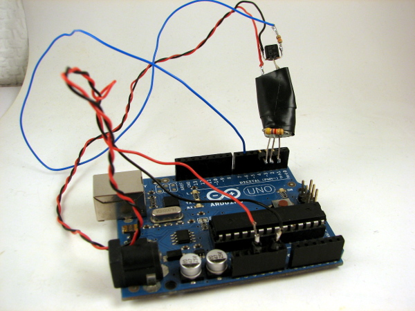
In control theory, the system under control is called a “plant”. My plant consists of a microcontroller, a DS18B20 temperature sensor and a resistor as a heater. Microcontroller pulses current through the resistor by applying pulse width modulated signal to a base of a transistor - that is called control signal. Temperature that is measured by the sensor is called the output of the system.

Modelling

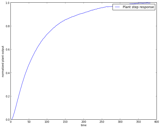
## Step response

Step response is a reaction of a system to the maximum signal level at its input. In my case this was PWM signal on a microcontroller. I chose my maximum to be 128 as it keeps the resistor from smoking and leaves the system a bit of hump behind it, if PID algorithm chooses to overdrive the control signal.

Impulse response

Impulse response is the derivative of the step response.

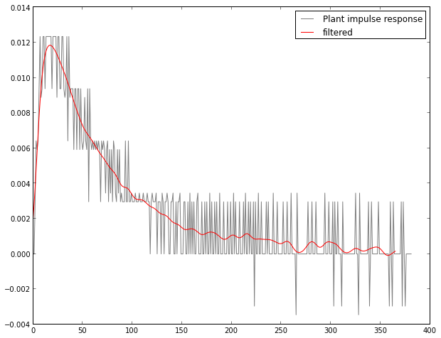
Impulse response is everything there is to be known about the system. It fully describes the possible behaviour of the system (provided some limitations - system has to be linear for this to work). To predict the behaviour of the system, for every discrete input value you have to multiply the impulse response by Dirac delta, scaled to input value, to get the ouput; and then on the next input, shift the previous output to right and add new output on the top, so impulse responses overlap on top of each other while time passes. This is called convolution.

Convolving impulse response with Dirac delta means applying full power to a system. Test the impulse response by convolving it with Dirac delta and compare it to our step response.

#convolve impuse reponse with 1. 1 * ir = y
for i in idx(y):
    for j in idx(ir):
        output[i+j] = output[i+j] + 1 * ir[j]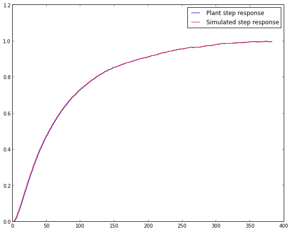

Nothing spectacular if you look at the math, but the result is really important, because now I can model my plant in software pretty accurately.

#this function processes one controll step at time t
def processStep(t, scaling):
    for j in idx(irFiltered):
        output[t+j] = output[t+j] + irFiltered[j] * scaling

PID algorithm

For my PID controller I’ve just used the first hit on the web search when looking for “PID Python”. It’s a bog standard PID implementation without any bells or whistles.

def update(self,current_value):
	"""
	Calculate PID output value for given reference input and feedback
	"""

	self.error = self.set_point - current_value

	self.P_value = self.Kp * self.error
	self.D_value = self.Kd * ( self.Derivator - current_value)
	self.Derivator = current_value

	self.Integrator = self.Integrator + self.error

	if self.Integrator > self.Integrator_max:
		self.Integrator = self.Integrator_max
	elif self.Integrator < self.Integrator_min:
		self.Integrator = self.Integrator_min

	self.I_value = self.Integrator * self.Ki

	PID = self.P_value + self.I_value + self.D_value
	if PID > 1:
		PID = 1
	if PID < 0:
		PID = 0
	return PID

Optimization

Error measure

To find an optimal solution, we need to have a way to estimate the controller performance. I’ve tried three estimation approaches with slightly different results, the final one I’ve chosen is called Integral of Time Absolute Error - it penalizes error the more the later it occurs.

def evaluate(p, setpoint):
    global output
    ITAE = 0
    MSE = 0
    IAE = 0
    output = np.zeros(150 + len(ir))
    controls = np.zeros(150)
    p.setPoint(setpoint)
    control = 0
    for t in range(0, 150):
        controls[t] = control
        processStep(t, control)
        control = p.update(output[t])
        error = output[t] - setpoint
        ITAE = ITAE + t * abs(error)
        MSE = MSE + error**2
        IAE = IAE + abs(error)
    output = output[:-len(ir)]
    MSE = MSE / 150
        
    return ITAE

Evolution

I start with a random population of PID controllers. On each evolution step a third of the population dies, then the best specimen mates with the better half of the remaining population and the rest mate and mutate randomly.

def nextGeneration(population):
    population.sort(key=lambda individual: individual.getFitness())
    population = population[:-POPULATION/3*2] #part of population dies
 
    alpha = population[0]
    #alpha female mates with the best without mutation
    for i in range(0, POPULATION/3 - 1):
        mama = alpha
        papa = population[int(rand() * len(population))]
        t = rand()
        if 0 < t <= 0.33:
            P = papa.Kp
            I = mama.Ki
            D = mama.Kd
        elif 0.33 < t <= 0.66:
            P = mama.Kp
            I = papa.Ki
            D = mama.Kd
        else:
            P = mama.Kp
            I = mama.Ki
            D = papa.Kd
        population.append(pid.PID(P, I, D))

    #all the other mate randomly and mutate a bit
    for i in range(0, POPULATION/3 - 1):
        papa = population[int(rand() * len(population))]
        mama = population[int(rand() * len(population))]
        t = rand()
        if 0 < t <= 0.33:
            P = papa.Kp + mutation(MAX_P * MUTATION_SCALE)
            I = mama.Ki + mutation(MAX_I * MUTATION_SCALE)
            D = mama.Kd + mutation(MAX_D * MUTATION_SCALE)
        elif 0.33 < t <= 0.66:
            P = mama.Kp + mutation(MAX_P * MUTATION_SCALE)
            I = papa.Ki + mutation(MAX_I * MUTATION_SCALE)
            D = mama.Kd + mutation(MAX_D * MUTATION_SCALE)
        else:
            P = mama.Kp + mutation(MAX_P * MUTATION_SCALE)
            I = mama.Ki + mutation(MAX_I * MUTATION_SCALE)
            D = papa.Kd + mutation(MAX_D * MUTATION_SCALE)
        population.append(pid.PID(P, I, D))
    
    #just for the kicks add a random one
    population.append(pid.PID(rand() * MAX_P, rand() * MAX_I, rand() * MAX_D))
    
    #and one mutation of alpha personally
    P = alpha.Kp + mutation(MAX_P * MUTATION_SCALE)
    I = alpha.Ki + mutation(MAX_I * MUTATION_SCALE)
    D = alpha.Kd + mutation(MAX_D * MUTATION_SCALE)
    population.append(pid.PID(P, I, D))
        
    return population

I have to note that I’m aware there are zillions of evolutionary frameworks for Python over the net, but my point here was to try the most naive uninitiated approach just to see if it works and experience the limitations and issues firsthand.

Let it live!

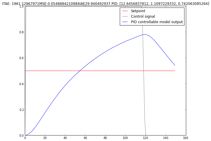
This is how the best controller out of a random population of 9 looks like

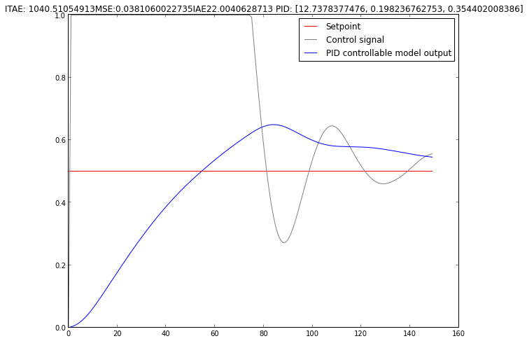
After something like 25 generations

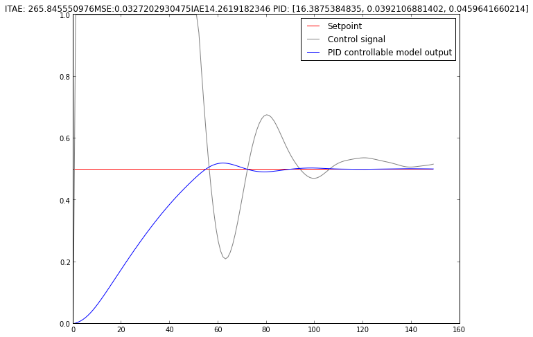
And the final winner after 50 generations

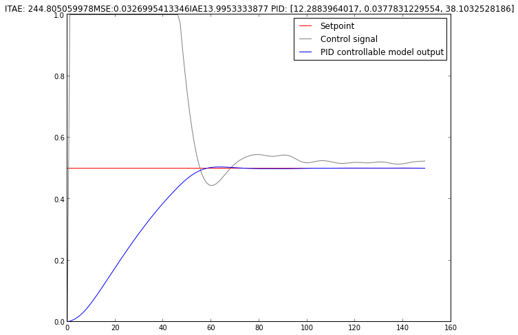
Making the population bigger and running simulation for more generations makes the result better - the overshoot is gone and there is almost no ringing. This one came out after running 50 generations with the population of 180.

Let’s try it on the real plant!

Well, remember, we had a real plant we are modelling. The whole point of the excercise was to determine PID coefficients for a real plant.

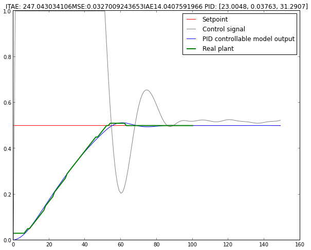
The green line on a plot is the output of my toy plant and it follows the model pretty closely. Suffice it to say, I’m very statisfied with the results and can’t wait to try this on a real kiln!

Conclusions

• Modelling of a system by using its impulse response to determine the optimal PID coefficients is a feasible approach.
• Genetic algorithms tend to be vulnerable to the problem of getting stuck in the local minima. Using a bigger population to “cover more teritory” is one way to overcome that.
• Evaluation fuction has to be carefully selected for a particular application - for some cases big overshoot can be an acceptable compromise when quickly reaching a setpoint is a priority and vice versa.
• The method can benefit from more insight into population dynamics - more diverse population could lead to better results when solution over several local minima has to be chosen.